A Technical Overview of YouTube Channel and Video Performance Analysis

2024/08/01 12:20 pm

Introduction

While AI advancements like recent Large Language Models (LLM) showcase remarkable technological progress, it’s crucial to underscore the need for a balanced approach that merges technical proficiency with domain-specific insights in data analytics. This project embodies this principle by attentively managing the quota limitations of the YouTube API and selecting and optimizing suitable combinations of machine learning and deep learning models for the Stacking Ensemble Classifier. Moreover, by leveraging interactive visualizations with Plotly and dashboards in PowerBI and Qlik Sense, the project enables us to derive meaningful insights into video content dynamics, which are practically applicable to improving video performance and audience engagement. Insights from the 2023 Kaggle AI Report and its best notebooks for best practices in ensemble modeling were instrumental in shaping the approach for this project.

The link to the repository of codes and dashboards of this project is in this link in my GitHub https://github.com/MortezaEmadi/YouTube-Channel-and-Video-Performance-Analysis-using-Google-API-and-Stacking-Ensemble-Classifier

However, here we will delve into the problem and also show how I have tried to develop the project with different tools to make it a real-world solution.

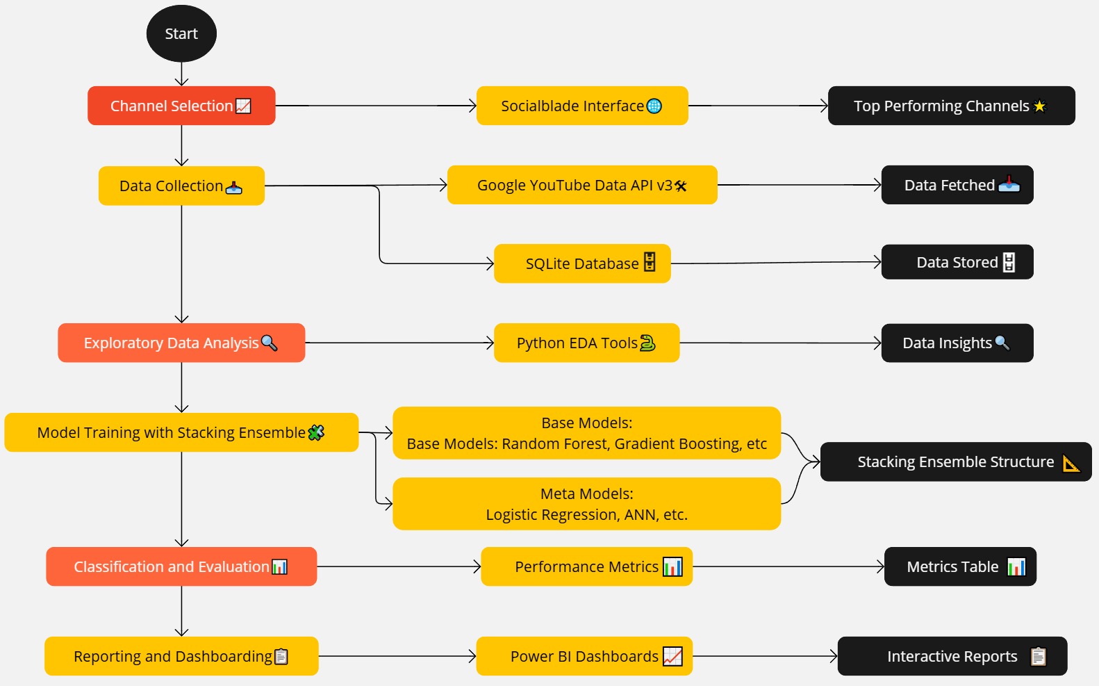
Fig. 1: Technical model development diagram.

◦ Introduction
◦ Research Problem
◦ Data Collection
◦ Exploratory Data Analysis (EDA)
◦ Feature Selection: Why Embedded Methods?
◦ Sentiment & Subjectivity Analysis with Relevance to Video Engagement
◦ Denoising Auto-Encoder (DAE) for Representation Learning in Tabular Data
- ◦ ◦ Swap Noise
- ◦ ◦ GaussRank Normalization
◦ Stacking Ensemble Structure
- ◦ ◦ Experimenting with Different Base and Meta-Models
- ◦ ◦ Optimizing Each Base and Meta-Model Candidate
- ◦ ◦ Optuna for Hyperparameter Optimization
- ◦ ◦ Passthrough vs Non-Passthrough in Stacking Ensemble
- ◦ ◦ Avoiding Data Leakage
- ◦ ◦ Non-Working Approaches
◦ PowerBI and Qlik Sense Dashboards
◦ ◦ Dashboard Visualizations
◦ Results of Ensemble Method
◦ References and Further Reading

Research Problem

Imagine you’re a broadcaster or an MOOC developer looking to understand how “Educational” video streamers perform. You might want to analyze audience engagement across various topics, such as DIY projects versus Social Science discussions, and understand how video duration impacts viewer interaction. YouTube’s Analytics dashboard is robust but limited in scope, especially when it comes to analyzing competitors’ data. This project uses the Google YouTube Data API v3 to extract valuable insights, focusing on engagement rates, video duration, upload frequency, and audience sentiment.

Data Collection

Google YouTube Data API v3: To collect the necessary data, I utilized the Google YouTube Data API v3. This API allows access to comprehensive metadata for both videos and channels. However, using this API comes with several challenges:

Quota Limits: The API has strict quota limits, restricting the amount of data that can be fetched within a given period.
Data Accessibility: Some features and data points are not accessible due to API restrictions.

Error Handling and Quality Data Storage: Given the quota limits and potential errors when accessing the API, robust error handling was implemented to ensure data quality and integrity. Data was stored in an SQLite database for efficient access and management. Here’s an overview of the error handling and data storage strategy:

Error Handling: Implemented retries and logging for API requests to handle temporary failures.
Data Validation: Ensured that fetched data met quality standards before being stored.
SQLite Database: Used SQLite for storing channel and video metadata, providing a lightweight yet powerful database solution.

Despite these measures, the limited quota posed a significant challenge. To mitigate this, I have reached out to the Google Research team for a researcher authentication, which, if granted, would allow for higher quota limits and better access to data.

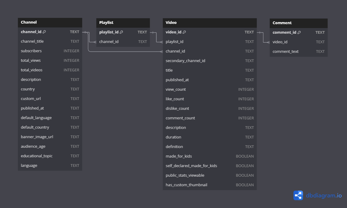
Fig. 2: ERD of the database after fetching data from Google API.

Exploratory Data Analysis (EDA)

Before interpreting the EDA results, it’s important to note that EDA is an observational study, showing associations that may involve lurking and confounding variables requiring further examination. The strategies suggested are based on a selective analysis of 95 channels within a subscriber range of 2 to 16 million.

In this analysis, we explored YouTube channels focused on educational topics within a limited subscriber range to provide a fair comparison for channels at similar growth stages. Channels are ordered by view count to highlight trends more effectively.

Insights:

Subscribers Distribution: Channels have subscribers ranging from 1.51 million to 4.55 million.
Total Views Distribution: Views range from approximately 286 million to 829 million. The average total views are around 473 million, with a high standard deviation of 142 million, indicating diverse engagement levels.
Correlation Analysis: A moderate positive correlation (0.64) between subscribers and total views suggests that more subscribers generally lead to more views. The low correlation between total views and total videos (-0.05) shows that having more videos does not necessarily result in higher views.
Publication Years: Most channels were created between 2010 and 2014, showing similar growth levels. Notable exceptions include newer channels achieving significant engagement.

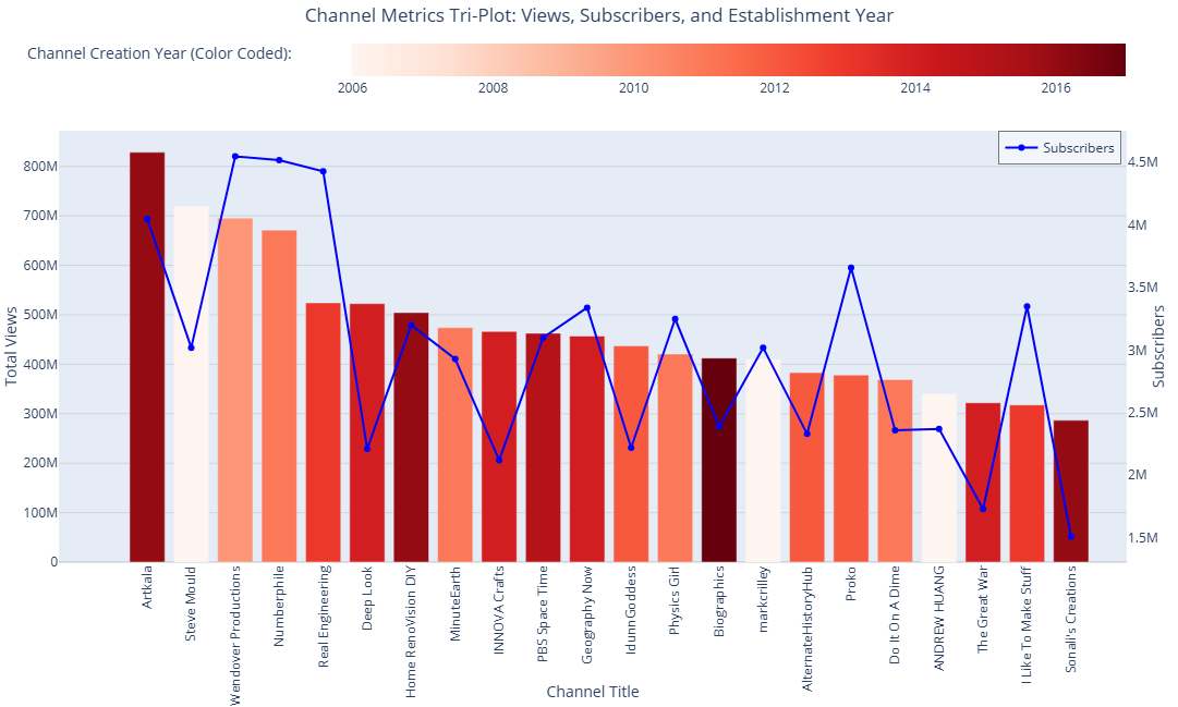
Fig. 3: Channels metrics plot with total view, total subscriber, and creation year.

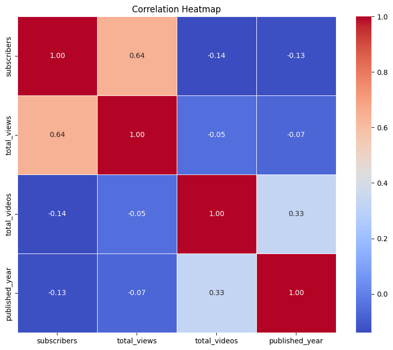
Fig. 4: Correlation heatmap of the main factors of the channels.

Notable Channels:

Artkala: Leading in total views (828 million) and substantial subscribers (4.05 million), showcasing the appeal of DIY content despite being relatively new (2016).
Biographics: The newest channel (2017) with 413 million views and 2.39 million subscribers, highlighting an effective content strategy in social sciences.

Conclusion: Channels with higher subscribers generally have higher total views, but more videos do not necessarily correlate with higher view counts. Channels established earlier, such as those from 2006, show enduring popularity. Additionally, DIY channels in the top quarter for view count and subscribers demonstrate rapid growth, indicating the potential of DIY content. The correlation analysis suggests that focusing on quality and engagement of content is more effective than merely increasing the number of videos.

Feature Selection: Why Embedded Methods Are Suitable

Embedded Methods: Embedded methods integrate feature selection directly into the model training process. This approach is particularly advantageous for small datasets with a high feature-to-row ratio because:

Efficiency: Embedded methods are generally more computationally efficient compared to wrapper methods, which involve training multiple models. This is crucial for small datasets where computational resources are limited.
Performance: Embedded methods strike a balance between computational cost and model performance. They are designed to select features that contribute the most to the model’s predictive power.
Overfitting: Embedded methods typically include regularization techniques that help reduce the risk of overfitting, which is a significant concern for small datasets like this project data.

Regularization Models like Ridge, Lasso, and Elastic Net can be used as embedded methods for feature selection. These models introduce a penalty term in the objective function during training to control the complexity of the model and encourage sparsity in the coefficient estimates. The resulting coefficients can then be used to assess the importance of features and perform feature selection.

Sentiment & Subjectivity Analysis with Relevance to Video Engagement

**Sentiment & Subjectivity Analysis:** Sentiment analysis is the process of determining the emotional tone behind a series of words, used to gain an understanding of the attitudes, opinions, and emotions expressed within an online mention. Subjectivity analysis, on the other hand, determines whether a piece of text is subjective (opinion-based) or objective (fact-based).

**Relevance to Video Engagement:** In the context of video engagement analysis, sentiment and subjectivity analysis can provide insights into how viewers feel about the content they are watching. For instance:

Positive Sentiments: Videos with titles and descriptions that have a positive sentiment tend to attract more viewers and receive higher engagement rates (likes, shares, comments). Positive emotions can encourage viewers to engage more with the content.
Negative Sentiments: Conversely, videos with negative sentiments might lead to lower engagement or provoke discussions and comments, depending on the nature of the content.
Subjectivity: Subjective content, which expresses personal opinions or emotions, can create a more engaging experience by resonating with viewers on a personal level. Objective content, presenting factual information, might appeal to viewers seeking knowledge or information.

By analyzing the sentiment and subjectivity of video titles, descriptions, and in the next phase even comments using TextBlob library, there are potentials to enhance viewer engagement. For instance, content creators might adjust the tone of their titles and descriptions regarding in which educational topic they are working to evoke a desired emotional response or foster a sense of community and discussion among viewers.

Denoising Auto-Encoder (DAE) for Representation Learning in Tabular Data

Auto-encoders have a long history and diverse applications, particularly for high-dimensional data such as images. These neural networks are designed to learn a compressed representation (encoding) of input data, typically for the purposes of dimensionality reduction or feature extraction. By reconstructing input data from its compressed form, auto-encoders can effectively identify and learn significant patterns in the data.

A denoising auto-encoder (DAE) is a specialized type of auto-encoder trained to remove noise from input data. The fundamental idea is to corrupt the input data with noise and train the auto-encoder to reconstruct the original, uncorrupted data. This approach helps the model learn more robust features and representations that are less sensitive to noise and variations in the data.

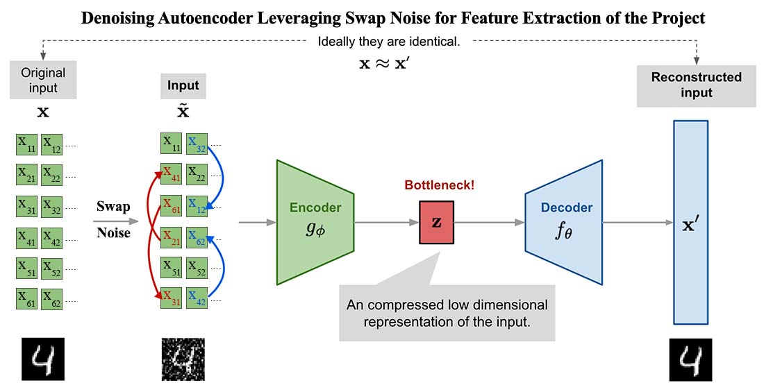
Fig. 5: Denoising Autoencoder with swap noise structure.

While DAEs are widely used for image data, recent best practices have demonstrated their effectiveness for tabular data with high feature-to-row ratios, such as in this project. DAEs are particularly useful for feature extraction and dimensionality reduction in small datasets, helping capture important patterns and relationships within the data.

In the case of unstructured data like images, text, or speech, there are numerous established tools to introduce noise. However, it is more challenging to add noise to structured tabular data because each variable may have a different range and distribution. For example, introducing Gaussian Noise to each variable requires determining an appropriate variance for each, which can be complex. Moreover, adding decimal noise to integer-only variables, such as counts, can distort the data.

Tailoring DAE for Tabular Data with Swap Noise and GaussRank Normalization: During recent best practices, using swap noise and GaussRank Normalization for DAEs has significantly improved their performance for tabular data. These techniques help enhance data augmentation and normalization, making DAEs powerful tools for representation learning in tabular datasets. The combination of these techniques helps overcome the challenges associated with training neural networks on small datasets, improving model robustness and generalization.

Key Techniques

Swap Noise:

Swap involves randomly swapping feature values within the same class to create synthetic data. This method increases data variability and helps prevent overfitting, especially in small datasets where additional training samples can significantly enhance model performance.
This type of noise substitutes existing values within the dataset, preventing the generation of out-of-place values. It is straightforward to use since it doesn’t require setting hyperparameters like mean or variance, and it is versatile across different variable distributions.

“`pyhton
import numpy as np

def swap_noise(df, swap_prob=0.1):
df_copy = df.copy()
for col in df.columns:
mask = np.random.rand(len(df)) < swap_prob
df_copy.loc[mask, col] = np.random.permutation(df[col].values[mask])
return df_copy

X_augmented = swap_noise(pd.DataFrame(X_normalized, columns=X.columns)).values
“`

Technical Insights:

Swap noise leverages the concept of data augmentation to artificially increase the size of the training dataset, which is crucial for improving model performance and generalization. By maintaining the class distribution and statistical properties of the original data, swap noise ensures that the synthetic samples are realistic and representative of the actual data distribution.

GaussRank Normalization:

Concept of GaussRank Normalization: GaussRank Normalization transforms features to follow a Gaussian distribution by ranking the data and applying the inverse Gaussian cumulative distribution function. This technique stabilizes the variance of features and improves the performance of algorithms that assume normally distributed data, such as neural networks.
In the context of DAEs, GaussRank Normalization helps neural networks learn more efficiently by normalizing ordinal variables into a Gaussian distribution, smoothing the optimization plane and improving training efficiency.

GaussRank Procedure:

Compute ranks for each value in a given column using argsort.
Normalize the ranks to range from -1 to 1.
Apply the inverse error function (erfinv) to transform the normalized ranks into a Gaussian distribution.

from tensorflow.keras.layers import Input, Dense
from tensorflow.keras.models import Model

input_dim = X_selected.shape[1]
encoding_dim = 24 # Adjust based on your needs

input_layer = Input(shape=(input_dim,))
encoder = Dense(encoding_dim, activation=’relu’)(input_layer)
decoder = Dense(input_dim, activation=’sigmoid’)(encoder)

autoencoder = Model(inputs=input_layer, outputs=decoder)
autoencoder.compile(optimizer=’adam’, loss=’binary_crossentropy’)
autoencoder.fit(X_augmented, X_augmented, epochs=50, batch_size=256, shuffle=True)

encoder_model = Model(inputs=autoencoder.input, outputs=encoder)
X_encoded = encoder_model.predict(X_selected)

Why DAE Works Well

Noise Reduction: By learning to remove noise from corrupted input data, DAEs create cleaner and more robust features.
Dimensionality Reduction: DAEs effectively reduce the number of features while preserving essential information, which is crucial for small datasets.
Enhanced Representation: The learned representations are often more meaningful and less redundant, improving the overall performance of downstream models.

So, the combination of these techniques helps overcome the challenges associated with training neural networks on small datasets, improving model robustness and generalization.

Stacking Ensemble Structure

Stacking ensemble is a powerful machine learning technique that combines multiple models (base models) to create a meta-model, which improves predictive performance. The base models are trained on the original dataset, and their predictions are then used as input features for the meta-model. This hierarchical approach leverages the strengths of different models to produce a more robust and accurate final prediction.

Experimenting with Different Base and Meta-Models

Experimenting with various base and meta-models is essential to find the best combination that maximizes performance. Different base models such as XGBoost, AdaBoost, K-Nearest Neighbors (KNN), Logistic Regression, and Neural Networks were evaluated. The meta-model, which aggregates the predictions of the base models, was also varied to identify the optimal configuration.

Optimizing Each Base and Meta-Model Candidate

Optimization of hyperparameters for each base model and the meta-model is crucial for achieving the best performance. This was done using Optuna, a hyperparameter optimization framework that automates the process of finding the best parameters efficiently. Optuna uses techniques like Tree-structured Parzen Estimator (TPE) and pruning to expedite the search.

Passthrough vs Non-Passthrough in Stacking Ensemble

In stacking, passthrough refers to including the original features along with the base model predictions as input to the meta-model.

Passthrough Format: The meta-model receives both the original features and the base model predictions. This can potentially improve performance by providing more information but may lead to overfitting if not handled correctly.
Non-Passthrough Format: The meta-model receives only the base model predictions. This approach reduces complexity and risk of overfitting but may miss out on useful information from the original features.

Avoiding Data Leakage

Avoiding data leakage in stacking ensembles is critical. This is achieved by generating out-of-fold predictions for the base models and using these predictions to train the meta-model. This ensures that the meta-model does not have access to the actual target values of the training data.

“`python
from sklearn.ensemble import StackingClassifier
from sklearn.model_selection import cross_val_predict

kf = KFold(n_splits=5, shuffle=True, random_state=42)
base_models = [(‘rf’, RandomForestClassifier()), (‘knn’, KNeighborsClassifier())]
meta_model = LogisticRegression()

#Generate out-of-fold predictions

oof_preds = np.zeros((X_train.shape[0], len(base_models)))

for i, (name, model) in enumerate(base_models):
oof_preds[:, i] = cross_val_predict(model, X_train, y_train, cv=kf)

#Train meta-model on out-of-fold predictions

meta_model.fit(oof_preds, y_train)

#Generate predictions for test set

test_preds = np.column_stack([
model.fit(X_train, y_train).predict(X_test)
for name, model in base_models
])
final_predictions = meta_model.predict(test_preds)
“`

Non-Working Approaches

Despite extensive experimentation, not all techniques yielded positive results. Notably, the use of polynomial features and LightGBM did not improve the model’s performance and, in some cases, worsened it. Polynomial features introduced multicollinearity, making the model less stable. LightGBM struggled with convergence issues, particularly on the small dataset, leading to suboptimal performance compared to XGBoost.

In small datasets, XGBoost often outperforms LightGBM due to its robust handling of overfitting. XGBoost incorporates a more regularized model formalization to control overfitting, making it more suitable for small datasets where overfitting is a significant concern. Additionally, XGBoost’s tree pruning algorithm is more conservative, which helps in achieving better performance in small datasets.

Key Differences:

Regularization: XGBoost has a more sophisticated regularization mechanism compared to LightGBM.
Tree Pruning: XGBoost uses a max depth parameter to limit the tree size, whereas LightGBM uses a leaf-wise growth strategy, which can lead to deeper trees and potential overfitting in small datasets.

PowerBI and Qlik Sense Dashboards

To visualize the data and insights generated from the project, a comprehensive dashboard was developed using both PowerBI and Qlik Sense. These dashboards provide an interactive and intuitive way to explore the analysis results.

Dashboard Visualizations

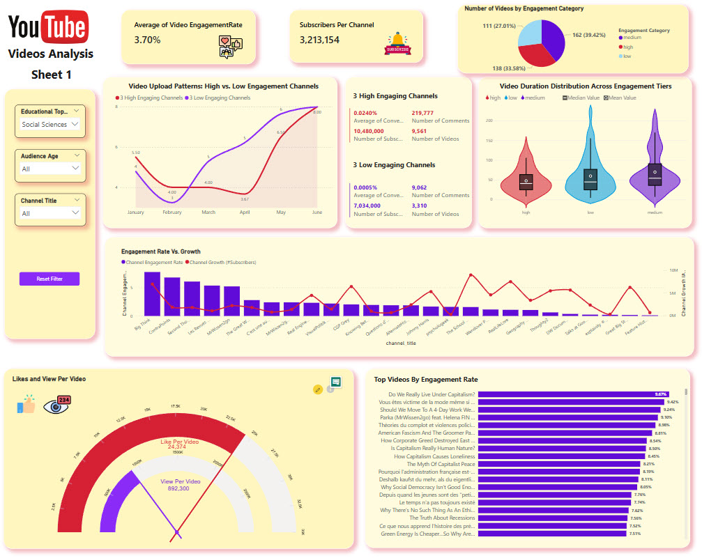
The dashboard includes several insightful visualizations designed to help users understand various aspects of video engagement:

Slicers for Filtering:
- Educational Topic: Allows users to filter videos based on different educational topics.
- Audience Age Group: Filters videos by the age group of the audience.
- Channels: Enables users to select specific YouTube channels for detailed analysis.
Pie Charts:
- Shows the distribution of engagement rates across different videos, helping to identify which videos are more engaging.
- Pie charts illustrating the ratios of views and likes per video to gauge audience response.
Gauges:
- Includes gauges for key performance indicators such as views per video and likes per video, providing a quick snapshot of video performance.
Video Duration Analysis:
- Analyzes video durations categorized by high, medium, and low engagement levels to identify trends and optimal video lengths.
Upload Frequency Comparison:
- Compares the upload frequency of the most engaging videos with the least engaging ones, offering insights into effective content strategies.

———————————————————

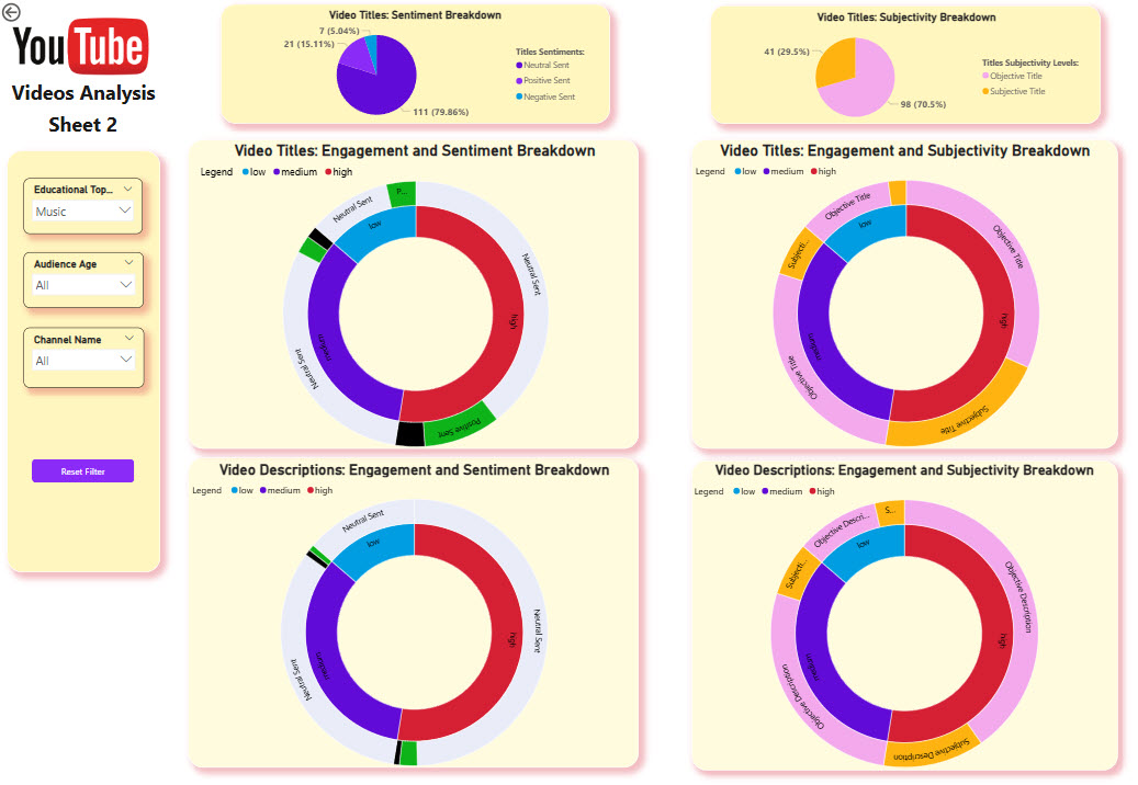
Fig. 6: PowerBI Dashboard in two sheets

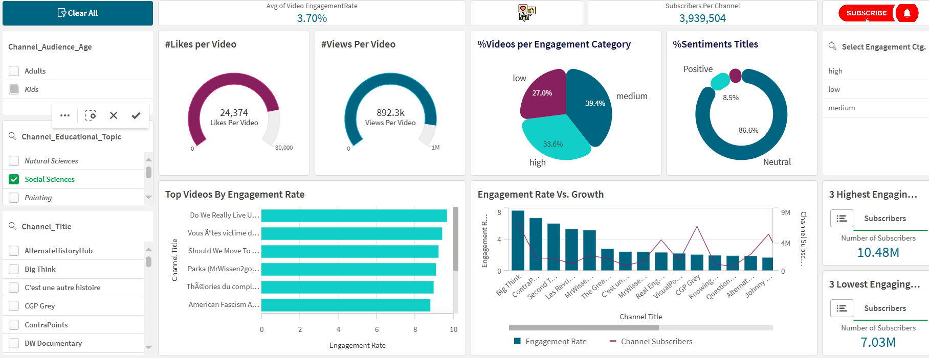
Fig. 7: Qlik Sense Dashboard

Additional enhancements are being prepared, such as visualizations for sentiment distributions of video titles and descriptions, which will further enrich the dashboard’s insights.

Results of Ensemble Method

In this project, the best model configuration consisted of using Random Forest, XGBoost as a gradient-boosted decision tree, KNN and MLP as the base models and XGBoost again as the meta-learner with the “passthrough” mode enabled. This configuration significantly improved the performance over individual models.

Best Base Model Performances:

Random Forest: Achieved an accuracy of 0.6750.
Gradient Boosting: Achieved an accuracy of 0.6729.

Ensemble Model Performance: The stacking ensemble method outperformed individual models, achieving an accuracy of 0.7273. This ensemble model demonstrated substantial improvements across various metrics, showcasing the effectiveness of combining multiple models.

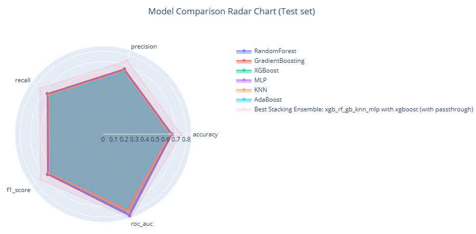
Fig. 8: Performance metrics of the ensemble model results in a radar diagram

For a detailed comparison and visualization of the enhancements in each classification criterion, refer to Fig. 8, which presents the improvements in a radar plot. This plot highlights the gains in accuracy, precision, recall, f1_score, and roc_auc, emphasizing the ensemble model’s superior performance.